One EC2 Box vs an EMR Cluster: Converting 256 GB of JSON to Parquet

Before a question ever reaches an NL2SQL pipeline, someone has to get the data into a shape worth querying. That work is unglamorous and it is where a surprising amount of time goes: reading raw exports, flattening nested structures, and landing the result as columnar files a query engine can scan quickly. This post is about that step, taken to AWS and measured rather than guessed.

The task: convert the Spotify Million Playlist Dataset from JSON to Parquet - one row per playlist, the nested track list kept intact as an array<struct> column - and do it in the cloud. The reflexive 2026 answer to "big data job" is spin up Spark, so I ran it two ways: EMR Spark (the distributed, scale-it-out approach) and a single large EC2 instance running the single-node engines (DuckDB, PyArrow, Polars). The interesting finding isn't which engine won. It's that the wall-clock time was governed almost entirely by disk throughput and the OS page cache - not cores, and not RAM.

TL;DR

• EMR Spark converted 150 GB in an ~11-minute step (~16-21 min end-to-end with provisioning), for about $0.35. Correct, but slower and costlier than a single node - the same 150 GB took ~4 minutes with DuckDB on one machine.
• A single EC2 box running DuckDB did 256 GB in 99 seconds on local NVMe - 8 million playlists - using ~7 GB of RAM. The whole exercise (two instances, three engines, two storage tiers) cost ~$2.28 on per-second billing.
• The single biggest lever wasn't the engine. On gp3 EBS, the identical DuckDB run took 143 s cache-hot and 264 s cache-cold. Swapping gp3 for local NVMe took it to 99 s on more data. You're often benchmarking your disk.
• Because DuckDB and PyArrow stream, RAM was never the constraint - which means a 32-64 GB laptop with an NVMe SSD does this job too, for $0.

The dataset is not the JSON you were expecting

The first surprise is the input format. The Million Playlist Dataset is delivered as 1,000 slice files per folder, and each slice is one pretty-printed JSON object:

{
  "info": { "slice": "0-999", ... },
  "playlists": [
    { "pid": 0, "name": "Throwbacks", "collaborative": "false",
      "modified_at": 1493424000, "num_tracks": 52,
      "tracks": [ { "pos": 0, "artist_name": "Missy Elliott", ... } ] },
    ... 999 more ...
  ]
}

It is not newline-delimited JSON. Each file is a single ~32 MB object whose playlists array has to be exploded into 1,000 rows, while the top-level info key is dropped. That detail trips up every engine's default reader, which assumes one JSON value per line. Getting each engine to read a multi-line single object is half the work.

The target schema is identical across all engines, so the outputs are directly comparable:

pid, name, collaborative (bool), modified_at, modified_at_ts (UTC timestamp),
num_tracks, num_albums, num_followers, num_edits, duration_ms, num_artists,
description, tracks (array<struct>)

To get real volume I copied the 30 GB set into N real folders (5 copies = 150-160 GB, 8 copies = 256 GB). "Real" matters: on a copy-on-write filesystem like XFS, cp defaults to --reflink=auto and makes instant clones that share blocks - a "160 GB" that's really 41 GB and reads entirely from cache, quietly invalidating the benchmark. cp --reflink=never forces genuine distinct bytes.

Round 1: EMR Spark, the "correct" big-data answer

I stood up an EMR cluster with a PySpark converter: read the JSON with multiLine=true, explode the playlists, repartition(110), write ZSTD Parquet to S3. There was a speed bump before any data moved: the EC2 vCPU quota. A fresh account gets 32 vCPU of Standard instances, and EMR counts every node against it. My first shape asked for 68 vCPU and died at provisioning with TERMINATED_WITH_ERRORS. The shape that fit was tiny:

CORE_COUNT=1  TASK_COUNT=0    # 1x m6a.xlarge primary + 1x m6a.4xlarge core = 20 vCPU

That's the first quiet lesson: a quota-capped Spark cluster is barely bigger than one machine. The result on 150 GB:

Stage	Time
Step (conversion only)	~11 min (05:18:56 → 05:29:56 UTC)
End-to-end (incl. provisioning)	~16-21 min

Output: 110 x ~120 MB ZSTD Parquet, ~13 GB, in S3. Correct - just slow. The same 150 GB on a single box with DuckDB took ~4 minutes. Spark was ~2.7x slower on raw processing and ~4-5x slower end-to-end once cluster spin-up is counted. Why the distributed engine lost on a job this size:

• Distributed overhead with none of the scale. Spark pays JVM startup, YARN scheduling, and a shuffle - repartition(110) moves all ~5M rows (nested tracks and all) across the network. On a 20-vCPU cluster you carry the entire distributed tax and get roughly one machine's parallelism back.
• Everything round-trips through S3. Every read and all 110 writes cross the wire; the single-node engines read and write local disk.

Cost. EMR bills the EC2 rate plus an EMR uplift, per second: the m6a.xlarge primary at $0.2160/hr combined and the m6a.4xlarge core at $0.8640/hr = $1.08/hr for the cluster. At ~16-21 min of life that's ≈ $0.35. Cheap in absolute terms, but slower and costlier than a single node - the theme of the whole study.

Round 2: one big EC2 box, and the I/O wall nobody mentions

I gave the single-node engines a real machine: m6a.8xlarge - 32 vCPU, 128 GB RAM - over 5 folders (160 GB) at 5 workers x 6 threads.

DuckDB's first pass finished in 143 seconds. Then I ran the others, then re-ran DuckDB on identical work - and it took 264 seconds. Same code, same data, same box, 1.8x slower.

Engine	Wall time	Notes
DuckDB (cache-hot)	143 s	data still in page cache from the cp
PyArrow	226 s
Polars	296 s	~65 GB RAM peak - materializes each folder before write
DuckDB (cache-cold)	264 s	run after the others churned the cache → disk-bound

The whole gap is the OS page cache. The first DuckDB run read its input from RAM (the cp had just left it there); by the second run, PyArrow and Polars had evicted it, so DuckDB went back to gp3 EBS at ~500 MB/s. And 160 GB can't fully cache in 128 GB of RAM.

That reframes the exercise. In htop, DuckDB used 6.50G/123G of RAM - almost nothing - yet the 32 cores mostly sat at 10-25%, starved, waiting on the disk. That's an I/O-bound run: plenty of CPU, plenty of RAM, and a disk that can't feed either.

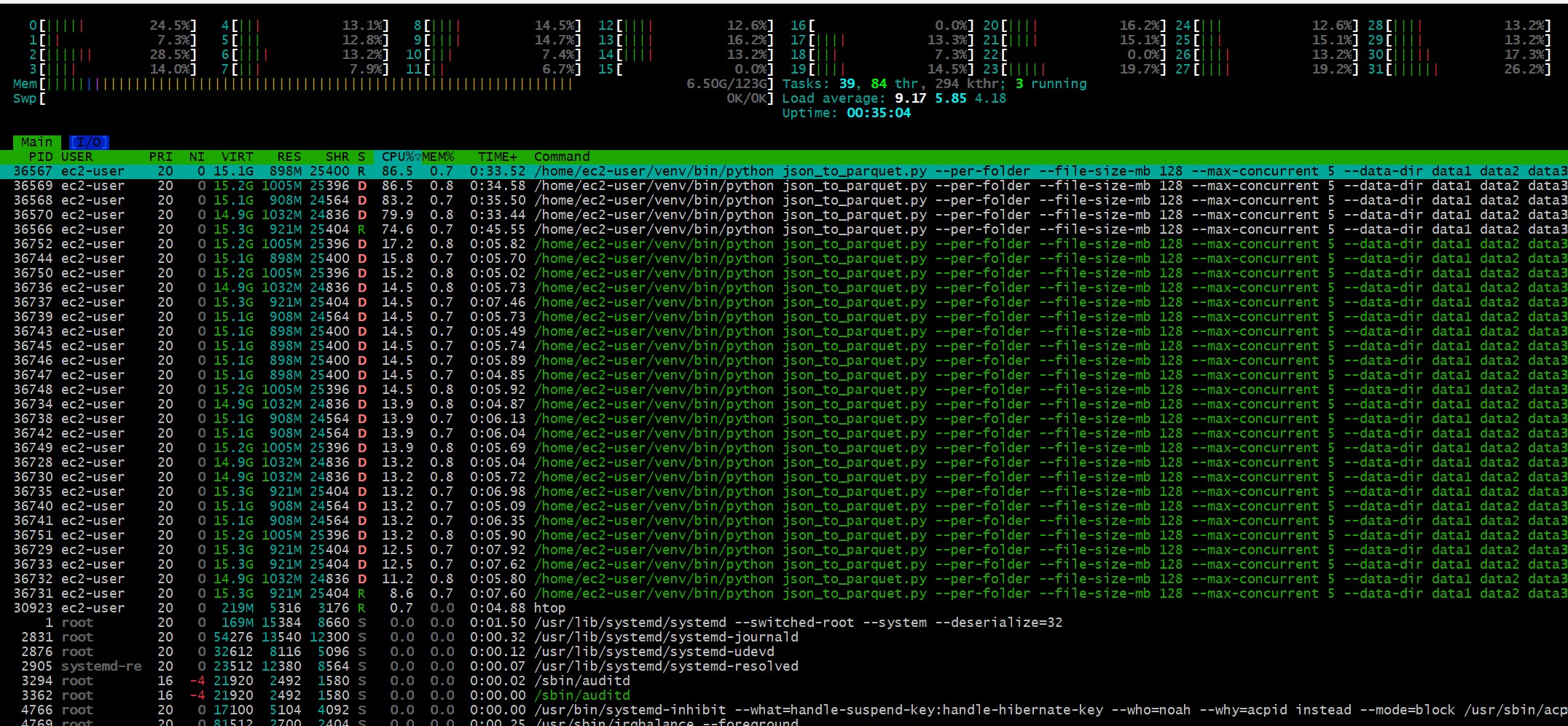
The benchmark you're running on a big read is often your disk, not your engine. A "faster" result can just be a warmer cache. Measure cold, and know which runs were hot.

Round 3: kill the I/O wall with local NVMe

If the disk is the ceiling, raise the disk. I moved to m6id.8xlarge - same 32 vCPU / 128 GB, but with 1.9 TB of local NVMe (~2.6 GB/s) instead of network-attached gp3. I staged 8 folders (256 GB) on the NVMe and ran everything 8-wide:

Engine	Wall time	Output	Peak RAM	Notes
DuckDB	99 s	21.0 GB	~7 GB	all 8 workers finished within 9 s
PyArrow	135 s	21.1 GB	-	streams batches
Polars (8-wide)	OOM	-	-	worker killed - 8 x ~15 GB > 123 GB
Polars (6-wide)	293 s	23.3 GB	~102 GB → 18 GB	eager concat spikes, then write phase drops

DuckDB did 256 GB in 99 seconds - ~2.6 GB/s effective, right at the NVMe ceiling - versus 264 s for 160 GB on cold gp3 (~0.6 GB/s). More data, less time, because the I/O wall was gone. Same engine, same ~7 GB footprint (5.31G/124G in htop) - but now all 32 cores pegged at ~100%. Nothing changed but the disk underneath. The extra RAM did nothing; the faster disk did everything.

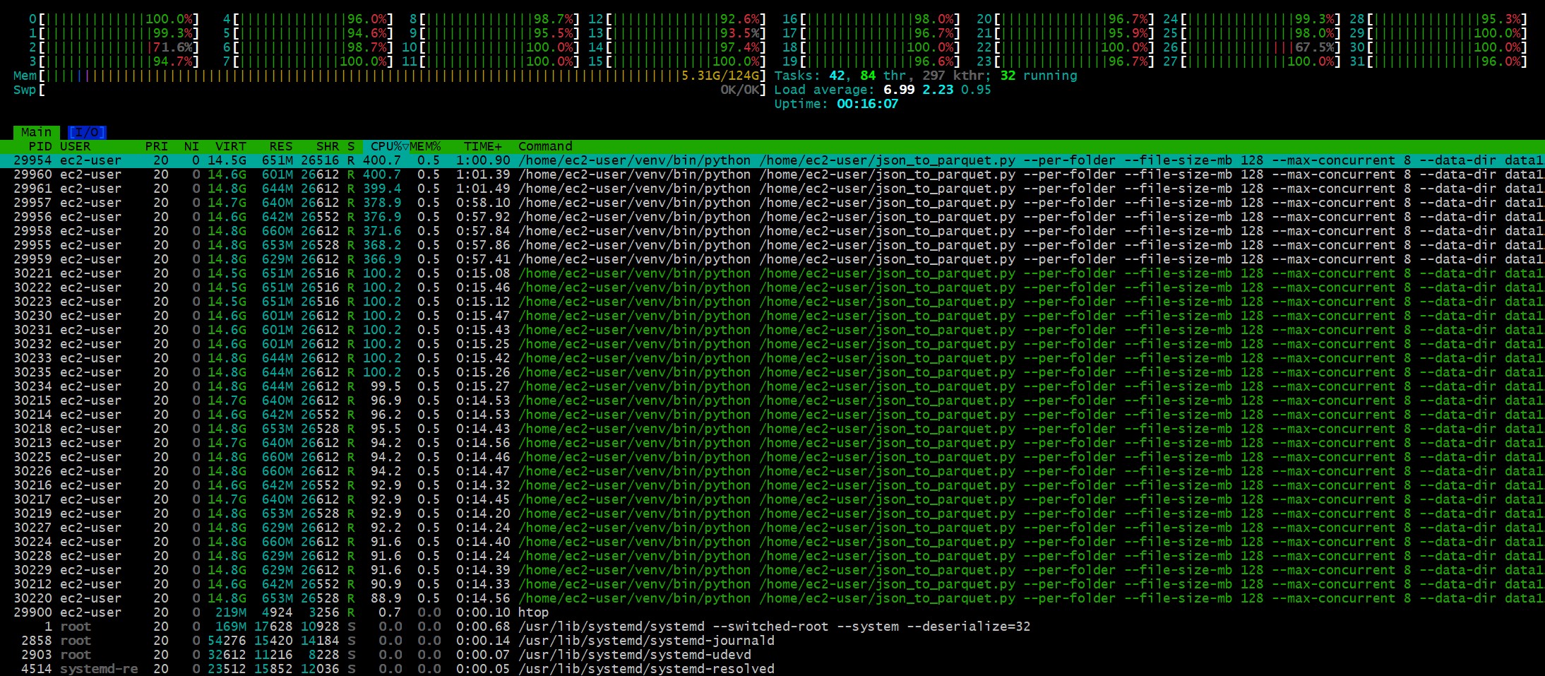
That's 8,000,000 playlists converted, tracks nested, in under two minutes on a single box.

Streaming vs materializing decides the memory story

Three engines, same job, wildly different memory behavior - and it's the whole reason concurrency scaled the way it did:

• DuckDB never held the dataset. ~7 GB whether processing 160 or 256 GB. It reads one file per thread, unnests, and streams Parquet out with preserve_insertion_order=false. memory_limit was not the speed lever; disk throughput was.
• PyArrow also streams, batch by batch, and scaled cleanly to 8-wide.
• Polars materializes. For this pretty-printed shape it has no lazy streaming scanner, so each worker reads its whole folder, explodes, and concats before writing - ~15 GB per worker. At 8-wide that's ~102 GB+ and the OOM killer stepped in; at 6-wide its trace spikes to ~102 GB during concat, then falls to ~18 GB in the write phase. On the same NVMe box DuckDB sat at 5.31 GB and Polars at 114G/124G - 21x the memory, same job.

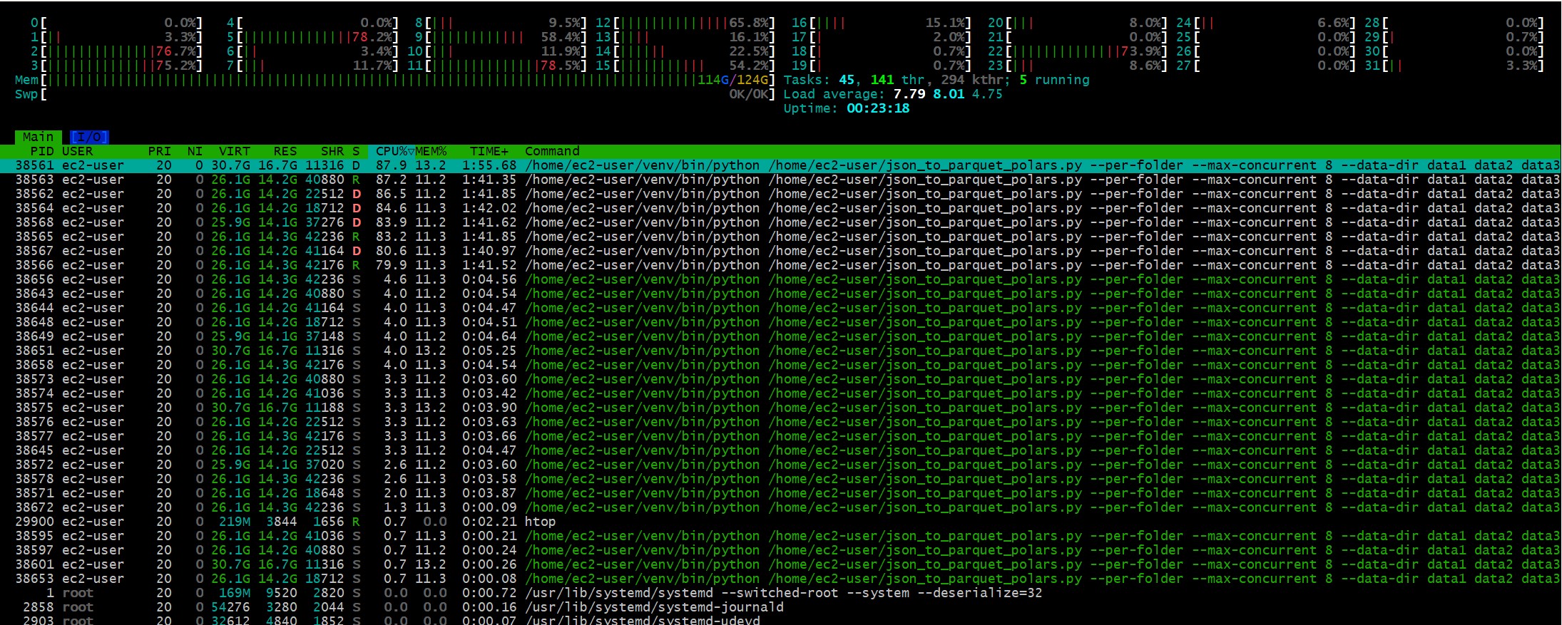
Throughput ranking held on both gp3 and NVMe: DuckDB > PyArrow > Polars.

The scoreboard: time and money

Run	Engine	Data	Wall (processing)	Cost
EMR Spark (20-vCPU)	Spark	150 GB	~11 min	~$0.35
EC2 m6a.8xlarge (gp3)	DuckDB	160 GB	143 s hot / 264 s cold	-
EC2 m6id.8xlarge (NVMe)	DuckDB	256 GB	99 s	-

The full EC2 cost - both instances, all three engines, per-second billing - was ≈ $2.28 (m6a.8xlarge $1.03 + m6id.8xlarge $1.26). Both instances were torn down; in-region S3↔EC2 transfer was free; the local NVMe is included in the hourly rate. The only lingering charge is ~$0.48/month for the Parquet output parked in S3. The whole study cost about the price of a coffee, because per-second billing only charges for the ~84 minutes the boxes were actually up.

You (probably) don't need the cloud for this at all

Here's the practical punchline, straight out of that 7 GB number: because DuckDB and PyArrow stream, RAM is not the constraint - disk is. DuckDB held ~7 GB converting 256 GB. That means the job fits a modest 32-64 GB laptop or desktop with fast local NVMe, no cloud required. The "300 GB of data needs a 128 GB machine" instinct is a materializing-engine assumption - true for Polars here, false for a streaming engine, where a 300 GB job and a 30 GB job use roughly the same memory. A sensible local recipe:

• Any 32-64 GB machine with an NVMe SSD. The 128 GB of cloud RAM sat unused; it bought nothing.
• Use DuckDB or PyArrow (streaming), with modest concurrency - the disk, not the cores, is the ceiling.
• Be careful going wide with Polars (or any materialize-then-write engine): ~15 GB per worker means 32 GB fits one or two workers.
• Watch the output disk, not RAM. 256 GB of JSON compresses to ~21 GB of ZSTD Parquet.

The cloud didn't win by having more memory - the 128 GB never mattered. It won, when it did, by having faster disk than gp3. Give a local machine the same NVMe and it does the same job for free.

Caveats (read these before quoting a number)

• Cross-machine comparisons mix hardware and engine. EMR-vs-single-node is systems, not engines in isolation - but that's the real decision you face.
• Timings are cold where it matters; the 143 s vs 264 s DuckDB gap is the page-cache effect, called out on purpose.
• Make real copies when you benchmark - CoW --reflink clones hand you a beautiful, meaningless number.
• The EMR cluster was quota-capped at 20 vCPU. A bigger cluster would close the gap on a big enough dataset - which is exactly when Spark earns its overhead.
• Instance-store NVMe is ephemeral (gone on stop/terminate) - it's for scratch and staging, not your only copy.

Closing

The tidy conclusion "engine X is fastest" didn't survive contact with 256 GB of JSON. What survived is more useful: for data that still fits one machine's disk throughput, the pragmatic answer isn't a cluster - it's a streaming engine on local NVMe. On AWS that was one m6id EC2 instance converting 8 million playlists in 99 seconds for pennies; off AWS it's the laptop already on your desk. Spark earns its keep when the data genuinely outgrows one machine. Until then, size the box to your disk, pick an engine that streams, and the single node wins on time, cost, and simplicity.